Difference between revisions of "OpenCV Tennis balls recognizing tutorial"
Andy753421 (talk | contribs) (→Processing) |
m (OpenCV moved to OpenCV Tennis balls recognizing tutorial) |
||
| (5 intermediate revisions by one other user not shown) | |||
| Line 1: | Line 1: | ||
| − | This tutorial demonstrates how to use an Elphel (or perhaps another) camera to perform some basic computer vision tasks, such as identifying objects. For this example, we will be recognizing tennis balls. | + | This tutorial demonstrates how to use an Elphel (or perhaps another) camera to perform some basic computer vision tasks, such as identifying objects. For this example, we will be recognizing tennis balls. A [[Image:Tennis.tar.gz|finished example]] is available for GNU/Linux systems. |
== Prerequisites == | == Prerequisites == | ||
| Line 10: | Line 10: | ||
== Image acquisition == | == Image acquisition == | ||
| + | [[Image:Tennis-input.jpg|thumb|Example input image]] | ||
| + | |||
The first step is to get some images into OpenCV and display them. This assumes you have AVLD and V4L already set up. Below is a fairly minimal example that captures and displays images. It can be compiled with '''gcc -o main main.c $(pkg-config --libs --cflags opencv)'''. | The first step is to get some images into OpenCV and display them. This assumes you have AVLD and V4L already set up. Below is a fairly minimal example that captures and displays images. It can be compiled with '''gcc -o main main.c $(pkg-config --libs --cflags opencv)'''. | ||
| Line 41: | Line 43: | ||
== Processing == | == Processing == | ||
=== Color space === | === Color space === | ||
| − | A good first step in many CV algorithms is to convert the image to HSV (or another similar color space). This | + | [[Image:Tennis-hsv.jpg|thumb|Example HSV output]] |
| + | |||
| + | A good first step in many CV algorithms is to convert the image to [http://en.wikipedia.org/wiki/HSL_and_HSV HSV] (or another similar [http://en.wikipedia.org/wiki/Color_space color space]). This makes picking out objects based on colors a bit simpler, as will be seen later. We'll make a copy of the original image so that we can display the original at the end. Note that OpenCV stores images in BGR format by default. | ||
<pre> | <pre> | ||
CvSize size = cvGetSize(img); | CvSize size = cvGetSize(img); | ||
| Line 49: | Line 53: | ||
=== Masks === | === Masks === | ||
| − | The next step is to select all pixels that we think might be part of a tennis ball. We'll do this based purely on their HSV values. OpenCV provides a InRanage function that can be used | + | [[Image:Tennis-mask.png|thumb|Example mask]] |
| + | |||
| + | The next step is to select all pixels that we think might be part of a tennis ball. We'll do this based purely on their HSV values. OpenCV provides a InRanage function that can be used to pick out pixels based on their values. This generates a [http://en.wikipedia.org/wiki/Mask_(computing) mask]; a binary image where the foreground pixels (white) were within the specified range. We're done with the HSV image after this, so we can free it's memory. | ||
| − | Picking the ranges for creating | + | Picking the ranges for creating masks is one of the more complicated parts of a CV algorithm. For now, manually tuning the ranges is easiest. You might also use one of the OpenCV machine learning algorithms to pick the ranges automatically. |
<pre> | <pre> | ||
| Line 61: | Line 67: | ||
=== Morphological operations === | === Morphological operations === | ||
| − | No matter how good your ranges are when generating a mask, there will almost always be noise in the mask. In our example, the white lines on the tennis ball don't show up because they don't fit the hue range. Much of this nose can be eliminated by using a series of morphological operations. Two commonly uses operation are [http://en.wikipedia.org/wiki/Opening_(morphology) opening] and [http://en.wikipedia.org/wiki/Closing_(morphology) closing], which are in turn comprised of [http://en.wikipedia.org/wiki/Dilation_(morphology) dilate] and [http://en.wikipedia.org/wiki/Erosion_(morphology) erode] operations. The table below summarizes these operations. | + | [[Image:Tennis-morph.png|thumb|Mask after morphological operations]] |
| + | |||
| + | No matter how good your ranges are when generating a mask, there will almost always be noise in the mask. In our example, the white lines on the tennis ball don't show up because they don't fit the hue range. Much of this nose can be eliminated by using a series of [http://en.wikipedia.org/wiki/Mathematical_morphology morphological operations]. Two commonly uses operation are [http://en.wikipedia.org/wiki/Opening_(morphology) opening] and [http://en.wikipedia.org/wiki/Closing_(morphology) closing], which are in turn comprised of [http://en.wikipedia.org/wiki/Dilation_(morphology) dilate] and [http://en.wikipedia.org/wiki/Erosion_(morphology) erode] operations. The table below summarizes these operations. | ||
{| border=1 | {| border=1 | ||
| Line 68: | Line 76: | ||
| Dilate || Expand the foreground | | Dilate || Expand the foreground | ||
|- | |- | ||
| − | | Erode || | + | | Erode || Contract the foreground (~ expand background) |
|- | |- | ||
| Close || Dilation followed by erosion, removes specks of background, fills in foreground areas. | | Close || Dilation followed by erosion, removes specks of background, fills in foreground areas. | ||
| Line 77: | Line 85: | ||
Morphological operations are performed with a [http://en.wikipedia.org/wiki/Structuring_element Structuring Element]. In computer vision, this is typically a oval or a rectangle of some specific size. Note that using rectangles results in faster code but can also cause poorer results. | Morphological operations are performed with a [http://en.wikipedia.org/wiki/Structuring_element Structuring Element]. In computer vision, this is typically a oval or a rectangle of some specific size. Note that using rectangles results in faster code but can also cause poorer results. | ||
| − | Below, we use a large rectangular structuring element along with a close to remove the black lines that show up in the tennis balls. Afterwards we perform an open with a smaller structuring element to eliminate some additional nose from the image. | + | Below, we use a large rectangular structuring element along with a close to remove the black lines that show up in the tennis balls. Afterwards, we perform an open with a smaller structuring element to eliminate some additional nose from the image. |
<pre> | <pre> | ||
IplConvKernel *se21 = cvCreateStructuringElementEx(21, 21, 10, 10, CV_SHAPE_RECT, NULL); | IplConvKernel *se21 = cvCreateStructuringElementEx(21, 21, 10, 10, CV_SHAPE_RECT, NULL); | ||
IplConvKernel *se11 = cvCreateStructuringElementEx(11, 11, 5, 5, CV_SHAPE_RECT, NULL); | IplConvKernel *se11 = cvCreateStructuringElementEx(11, 11, 5, 5, CV_SHAPE_RECT, NULL); | ||
| − | cvClose(mask, mask, se21); | + | cvClose(mask, mask, se21); // See completed example for cvClose definition |
| − | cvOpen(mask, mask, se11); | + | cvOpen(mask, mask, se11); // See completed example for cvOpen definition |
cvReleaseStructuringElement(&se21); | cvReleaseStructuringElement(&se21); | ||
cvReleaseStructuringElement(&se11); | cvReleaseStructuringElement(&se11); | ||
| Line 89: | Line 97: | ||
=== Hough transform === | === Hough transform === | ||
| − | The real work in finding tennis balls is done by a Hough transform. The specifics of this are beyond the scope of this tutorial. We'll just treat it as a black box function that finds circular objects in | + | The real work in finding tennis balls is done by a [http://en.wikipedia.org/wiki/Hough_transform Hough transform]. The specifics of this are beyond the scope of this tutorial. We'll just treat it as a black box function that finds circular objects in an input image. |
| − | The OpenCV Hough function performs a Canny edge detection on the input image before | + | The OpenCV Hough function performs a [http://en.wikipedia.org/wiki/Canny_edge_detector Canny edge detection] on the input image before the actual Hough transform. Due to this and the way the Hough transform works, it is beneficial to do quite a bit of smoothing to get a nice gradient around the edge of the circles before passing the image to the Hough function. Many of the parameters to the Hough function can also be tuned to provide better results. |
<pre> | <pre> | ||
| − | /* Copy mask into a | + | /* Copy mask into a grayscale image */ |
IplImage *hough_in = cvCreateImage(size, 8, 1); | IplImage *hough_in = cvCreateImage(size, 8, 1); | ||
cvCopy(mask, hough_in, NULL); | cvCopy(mask, hough_in, NULL); | ||
| Line 107: | Line 115: | ||
== Output == | == Output == | ||
| + | [[Image:Tennis-output.jpg|thumb|Example output on a particularly nice image]] | ||
| + | |||
| + | The output of the Hough function can then be used in a variety of ways. For now we'll just draw some circles and centers onto the original input image before displaying it. | ||
| + | <pre> | ||
| + | int i; | ||
| + | for (i = 0; i < circles->total; i++) { | ||
| + | float *p = (float*)cvGetSeqElem(circles, i); | ||
| + | CvPoint center = cvPoint(cvRound(p[0]),cvRound(p[1])); | ||
| + | CvScalar val = cvGet2D(mask, center.y, center.x); | ||
| + | if (val.val[0] < 1) continue; | ||
| + | cvCircle(img, center, 3, CV_RGB(0,255,0), -1, CV_AA, 0); | ||
| + | cvCircle(img, center, cvRound(p[2]), CV_RGB(255,0,0), 3, CV_AA, 0); | ||
| + | cvCircle(mask, center, 3, CV_RGB(0,255,0), -1, CV_AA, 0); | ||
| + | cvCircle(mask, center, cvRound(p[2]), CV_RGB(255,0,0), 3, CV_AA, 0); | ||
| + | } | ||
| + | </pre> | ||
== Acknowledgments == | == Acknowledgments == | ||
| + | Some of the code provided as part of this example was developed by Jon Nibert and Andy Spencer as part of the Image Recognition course taught at Rose-Hulman Institute of Technology. All examples are provided under the GNU GPLv3. | ||
Latest revision as of 01:56, 27 July 2010
This tutorial demonstrates how to use an Elphel (or perhaps another) camera to perform some basic computer vision tasks, such as identifying objects. For this example, we will be recognizing tennis balls. A File:Tennis.tar.gz is available for GNU/Linux systems.
Contents
Prerequisites
- OpenCV
- OpenCV is a C library designed to help with computer vision programs. It provides quite a few useful functions that can save a lot typing when performing operations on images.
- V4L/AVLD
- OpenCV provides a V4L API that can be used to acquire images from Elphel cameras. This is done using AVLD.
Image acquisition
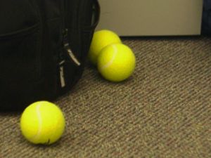
The first step is to get some images into OpenCV and display them. This assumes you have AVLD and V4L already set up. Below is a fairly minimal example that captures and displays images. It can be compiled with gcc -o main main.c $(pkg-config --libs --cflags opencv).
#include <opencv/cv.h>
#include <opencv/highgui.h>
#include <X11/keysym.h>

int main(int argc, char **argv)
{
	/* Start the CV system and get the first v4l camera */
	cvInitSystem(argc, argv);
	CvCapture *cam = cvCreateCameraCapture(0);

	/* Create a window to use for displaying the images */
	cvNamedWindow("img", 0);
	cvMoveWindow("img", 200, 200);

	/* Display images until the user presses q */
	while (1) {
		cvGrabFrame(cam);
		IplImage *img = cvRetrieveFrame(cam);
		cvShowImage("img", img);
		if (cvWaitKey(10) == XK_q)
			return 0;
		cvReleaseImage(&img);
	}
}
Processing
Color space
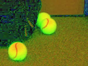
A good first step in many CV algorithms is to convert the image to HSV (or another similar color space). This makes picking out objects based on colors a bit simpler, as will be seen later. We'll make a copy of the original image so that we can display the original at the end. Note that OpenCV stores images in BGR format by default.
	CvSize size = cvGetSize(img);
	IplImage *hsv = cvCreateImage(size, IPL_DEPTH_8U, 3);
	cvCvtColor(img, hsv, CV_BGR2HSV);
Masks
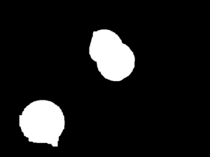
The next step is to select all pixels that we think might be part of a tennis ball. We'll do this based purely on their HSV values. OpenCV provides a InRanage function that can be used to pick out pixels based on their values. This generates a mask; a binary image where the foreground pixels (white) were within the specified range. We're done with the HSV image after this, so we can free it's memory.
Picking the ranges for creating masks is one of the more complicated parts of a CV algorithm. For now, manually tuning the ranges is easiest. You might also use one of the OpenCV machine learning algorithms to pick the ranges automatically.
	CvMat *mask = cvCreateMat(size.height, size.width, CV_8UC1);
	cvInRangeS(hsv, cvScalar(0.11*256, 0.60*256, 0.20*256, 0),
	                cvScalar(0.14*256, 1.00*256, 1.00*256, 0), mask);
	cvReleaseImage(&hsv);
Morphological operations
No matter how good your ranges are when generating a mask, there will almost always be noise in the mask. In our example, the white lines on the tennis ball don't show up because they don't fit the hue range. Much of this nose can be eliminated by using a series of morphological operations. Two commonly uses operation are opening and closing, which are in turn comprised of dilate and erode operations. The table below summarizes these operations.
| Operation | Effect / Use |
|---|---|
| Dilate | Expand the foreground |
| Erode | Contract the foreground (~ expand background) |
| Close | Dilation followed by erosion, removes specks of background, fills in foreground areas. |
| Open | Erosion followed by dilation, removes specks of foreground, fills in background areas. |
Morphological operations are performed with a Structuring Element. In computer vision, this is typically a oval or a rectangle of some specific size. Note that using rectangles results in faster code but can also cause poorer results.
Below, we use a large rectangular structuring element along with a close to remove the black lines that show up in the tennis balls. Afterwards, we perform an open with a smaller structuring element to eliminate some additional nose from the image.
	IplConvKernel *se21 = cvCreateStructuringElementEx(21, 21, 10, 10, CV_SHAPE_RECT, NULL);
	IplConvKernel *se11 = cvCreateStructuringElementEx(11, 11, 5,  5,  CV_SHAPE_RECT, NULL);
	cvClose(mask, mask, se21); // See completed example for cvClose definition
	cvOpen(mask, mask, se11);  // See completed example for cvOpen  definition
	cvReleaseStructuringElement(&se21);
	cvReleaseStructuringElement(&se11);
Hough transform
The real work in finding tennis balls is done by a Hough transform. The specifics of this are beyond the scope of this tutorial. We'll just treat it as a black box function that finds circular objects in an input image.
The OpenCV Hough function performs a Canny edge detection on the input image before the actual Hough transform. Due to this and the way the Hough transform works, it is beneficial to do quite a bit of smoothing to get a nice gradient around the edge of the circles before passing the image to the Hough function. Many of the parameters to the Hough function can also be tuned to provide better results.
	/* Copy mask into a grayscale image */
	IplImage *hough_in = cvCreateImage(size, 8, 1);
	cvCopy(mask, hough_in, NULL);
        cvSmooth(hough_in, hough_in, CV_GAUSSIAN, 15, 15, 0, 0);

	/* Run the Hough function */
	CvMemStorage *storage = cvCreateMemStorage(0);
	CvSeq *circles = cvHoughCircles(hough_in, storage,
		CV_HOUGH_GRADIENT, 4, size.height/10, 100, 40, 0, 0);
	cvReleaseMemStorage(&storage);
Output
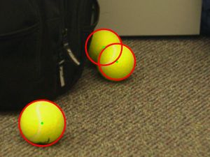
The output of the Hough function can then be used in a variety of ways. For now we'll just draw some circles and centers onto the original input image before displaying it.
	int i;
	for (i = 0; i < circles->total; i++) {
             float *p = (float*)cvGetSeqElem(circles, i);
	     CvPoint center = cvPoint(cvRound(p[0]),cvRound(p[1]));
	     CvScalar val = cvGet2D(mask, center.y, center.x);
	     if (val.val[0] < 1) continue;
             cvCircle(img,  center, 3,             CV_RGB(0,255,0), -1, CV_AA, 0);
             cvCircle(img,  center, cvRound(p[2]), CV_RGB(255,0,0),  3, CV_AA, 0);
             cvCircle(mask, center, 3,             CV_RGB(0,255,0), -1, CV_AA, 0);
             cvCircle(mask, center, cvRound(p[2]), CV_RGB(255,0,0),  3, CV_AA, 0);
	}
Acknowledgments
Some of the code provided as part of this example was developed by Jon Nibert and Andy Spencer as part of the Image Recognition course taught at Rose-Hulman Institute of Technology. All examples are provided under the GNU GPLv3.


